Autoscale + overlay + highlight

Recipes

Recipes combine several options into patterns that are useful in real figures.

Compare styles before choosing one

from plotnado import GenomicFigure
from plotnado.examples import REGION, signal
# signal() → DataFrame(chrom, start, end, value) — replace with a BigWig path/URL or DataFrame

fig = GenomicFigure(track_height=1.15)
fig.scalebar()
fig.bigwig(signal(phase=0.0), title="fill", style="fill", color="#1f77b4")
fig.bigwig(signal(phase=0.8), title="fragment", style="fragment", color="#d62728")
fig.bigwig(signal(phase=1.6), title="scatter", style="scatter", color="#2ca02c", scatter_point_size=10)
fig.bigwig(signal(phase=2.4), title="std", style="std", color="#9467bd")
fig.plot(REGION)

Render style comparisons in the docs or notebook instead of relying on remembered defaults.

from plotnado import GenomicFigure
from plotnado.examples import REGION, review_signal
# review_signal() → DataFrame(chrom, start, end, value) — replace with BigWig paths/URLs or DataFrames

fig = GenomicFigure(track_height=1.2)
fig.autoscale(True)
fig.highlight("chr1:1,032,000-1,046,000")
fig.highlight_style(color="#ffdd57", alpha=0.22)
fig.bigwig(review_signal(2.0), title="Control", autoscale_group="signal", color="#1f77b4")
fig.bigwig(review_signal(10.0, 1.2), title="Treatment", autoscale_group="signal", color="#d62728")
fig.overlay(
    [review_signal(5.5, 2.0), review_signal(6.5, 2.8)],
    title="Overlay",
    autoscale_group="signal",
    colors=["#2ca02c", "#9467bd"],
    alpha=0.55,
)
fig.plot(REGION)

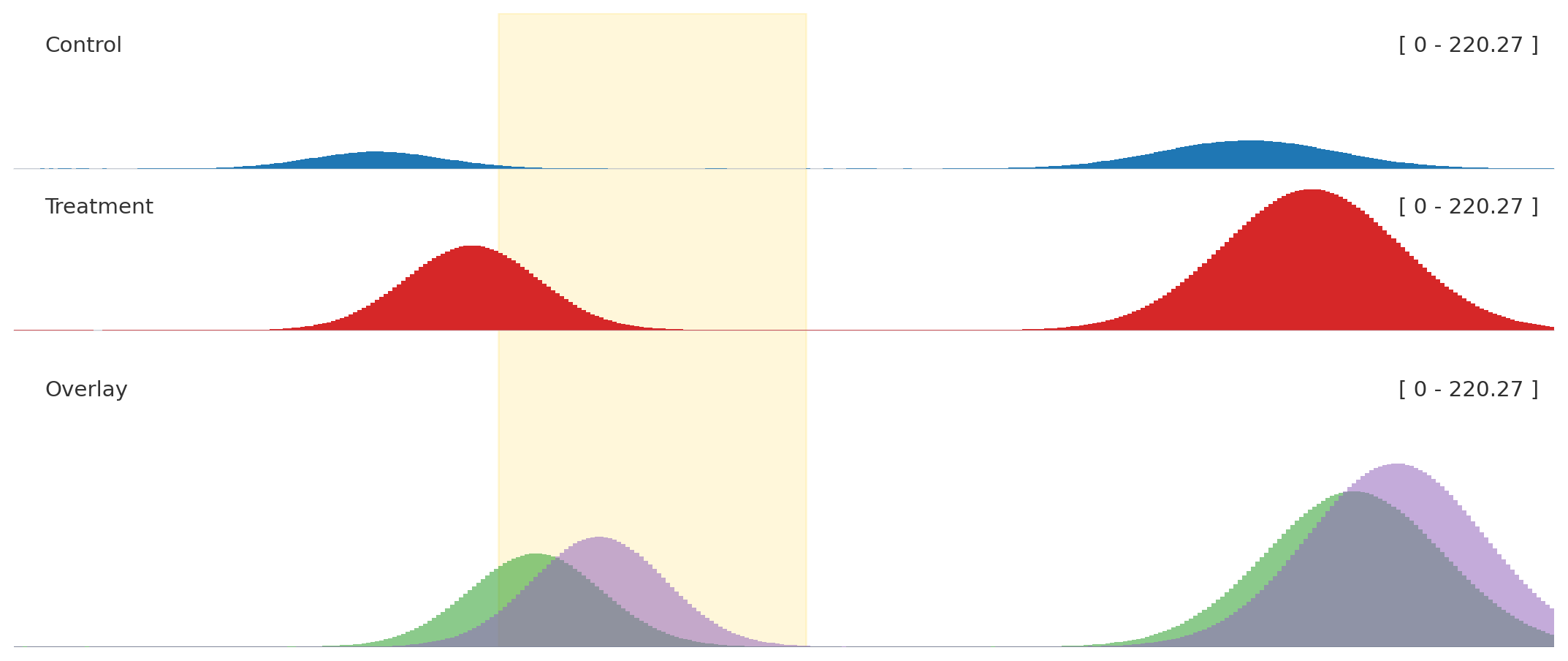
Use this when one overlay panel should sit next to ordinary signal tracks without drifting onto a different scale.

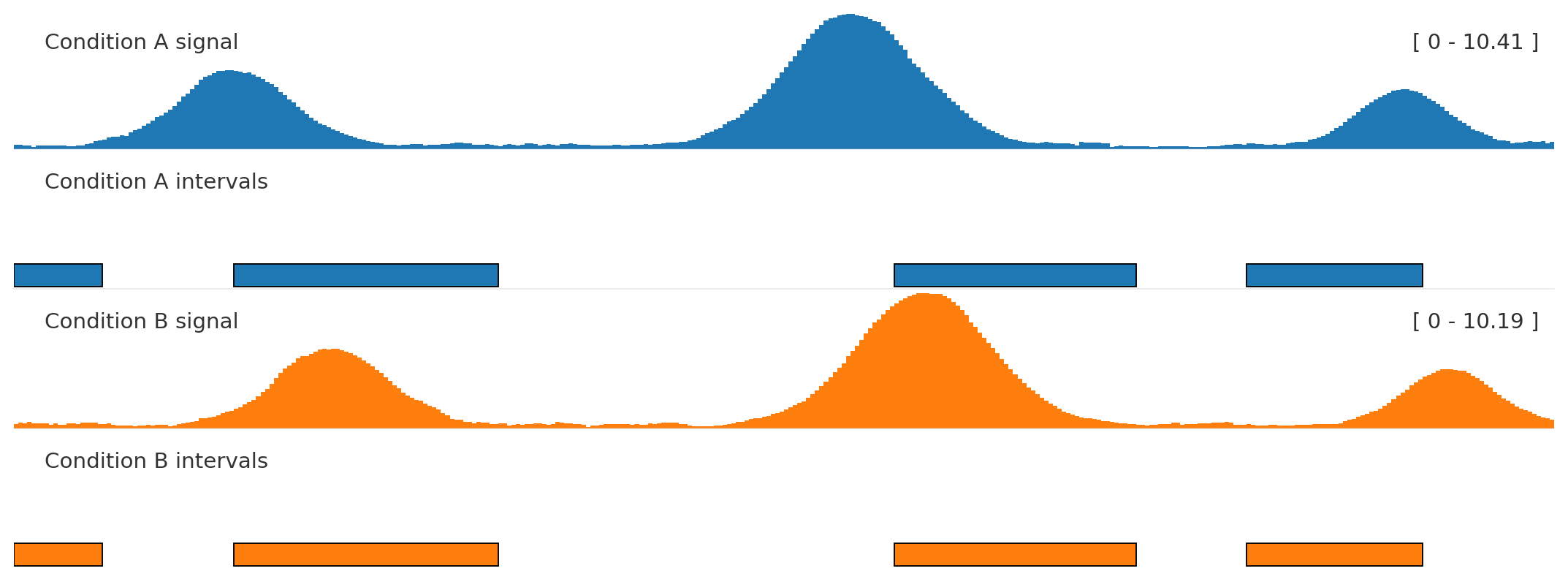
Autocolor + related interval tracks

from plotnado import GenomicFigure
from plotnado.examples import REGION, intervals, signal
# signal() → DataFrame(chrom, start, end, value) — replace with a BigWig path/URL or DataFrame
# intervals() → DataFrame(chrom, start, end, name) — replace with a BED/BigBed path, URL, or DataFrame

fig = GenomicFigure(track_height=1.05).autocolor("tab10")
fig.bigwig(signal(phase=0.0), title="Condition A signal", color_group="A")
fig.bed(intervals(), title="Condition A intervals", color_group="A", display="expanded")
fig.bigwig(signal(phase=1.1), title="Condition B signal", color_group="B")
fig.bed(intervals().assign(name=["b1", "b2", "b3", "b4"]), title="Condition B intervals", color_group="B", display="expanded")
fig.plot(REGION)

Use the same color_group for tracks that represent the same sample, condition, or assay.

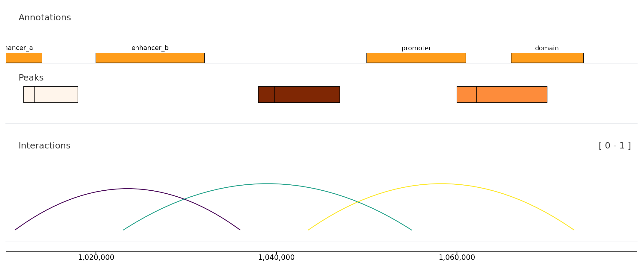
Interval and link context

from plotnado import GenomicFigure
from plotnado.examples import REGION, intervals, links, narrowpeaks
# intervals() → DataFrame(chrom, start, end, name) — replace with a BED/BigBed path, URL, or DataFrame
# narrowpeaks() → DataFrame(chrom, start, end, name, score, strand, signalValue, pValue, qValue, peak) — replace with a .narrowPeak path or DataFrame
# links() → DataFrame(chrom1, start1, end1, chrom2, start2, end2, score) — replace with a BEDPE path or DataFrame

fig = GenomicFigure(track_height=1.1)
fig.bed(intervals(), title="Annotations", display="expanded", show_labels=True)
fig.narrowpeak(narrowpeaks(), title="Peaks", color_by="signalValue", cmap="Oranges")
fig.links(links(), title="Interactions", color_by_score=True, cmap="viridis")
fig.axis()
fig.plot(REGION)

Use interval tracks for local annotations and links() for paired genomic anchors.

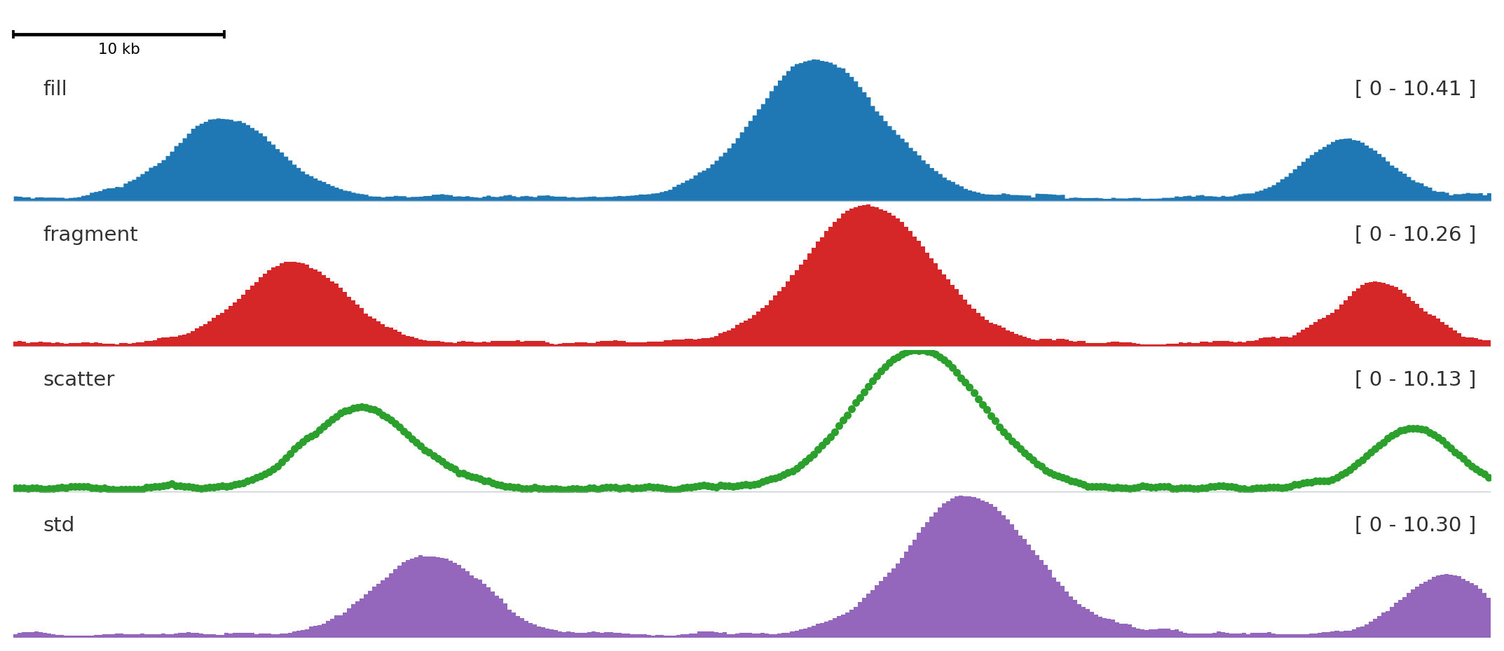
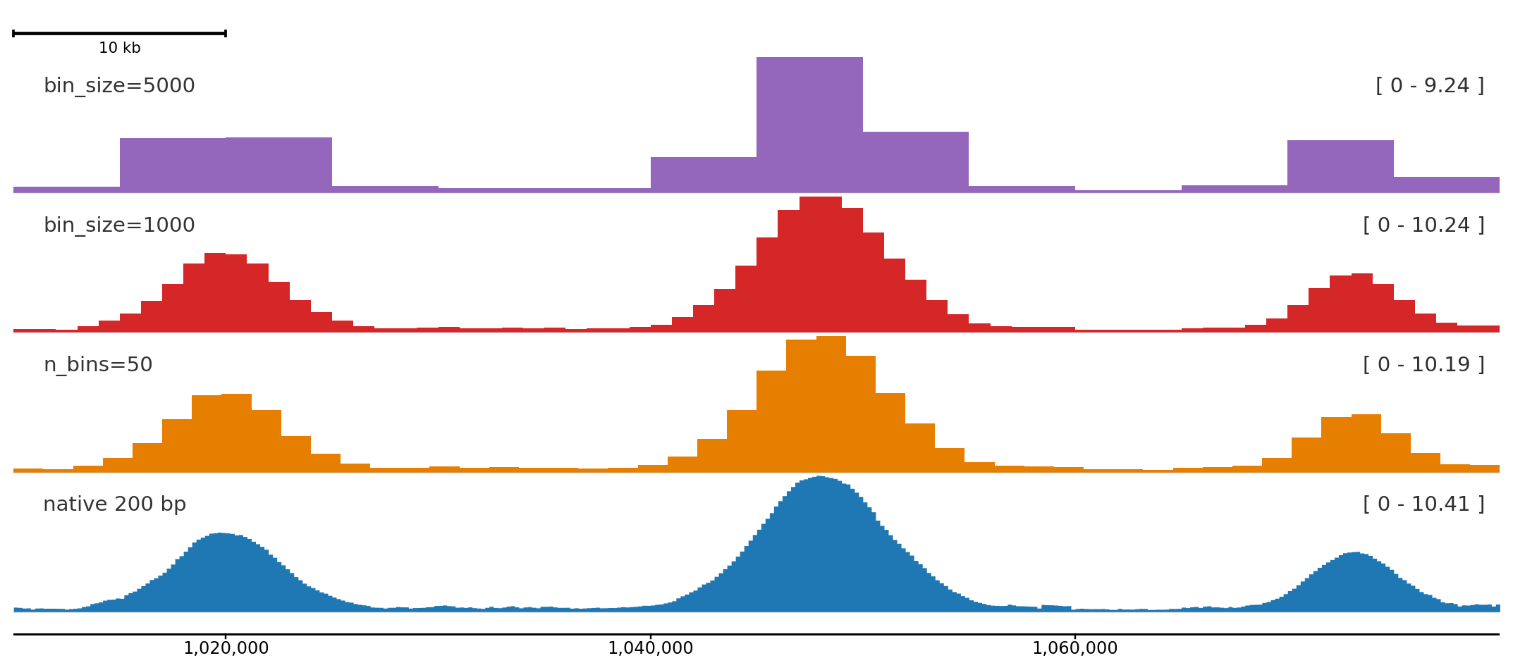
Control signal resolution

Use bin_size or n_bins to match bin width to the figure size and zoom level. Coarser bins reduce visual noise in wide regions; finer bins reveal peak shape at high zoom.

from plotnado import GenomicFigure
from plotnado.examples import REGION, signal
# signal() → DataFrame(chrom, start, end, value) — replace with a BigWig path/URL or DataFrame

fig = GenomicFigure(track_height=1.1)
fig.scalebar()
fig.bigwig(signal(), title="bin_size=5000", style="fill", color="#9467bd", bin_size=5000)
fig.bigwig(signal(), title="bin_size=1000", style="fill", color="#d62728", bin_size=1000)
fig.bigwig(signal(), title="n_bins=50",     style="fill", color="#e67e00", n_bins=50)
fig.bigwig(signal(), title="native 200 bp", style="fill", color="#1f77b4")
fig.axis()
fig.plot(REGION)

Same signal at three resolutions. bin_size keeps physical bin width fixed in bp; n_bins keeps the count fixed regardless of region size.

For BigWig files the rebinning is applied after fetching the native intervals, so there is no extra file I/O cost. For DataFrames the same weighted-average logic applies.

Save reusable figure definitions

fig.to_toml("figure.toml")
loaded = GenomicFigure.from_toml("figure.toml")
loaded.save("figure.png", region="chr1:1,000,000-1,100,000")

Run the maintained example suite with:

uv run python examples/run_examples.py