Worked Examples

Real-data examples using public BigWig and BigBed files from the Blueprint Epigenome Project (GRCh38). These examples require network access to the EBI FTP server.

---

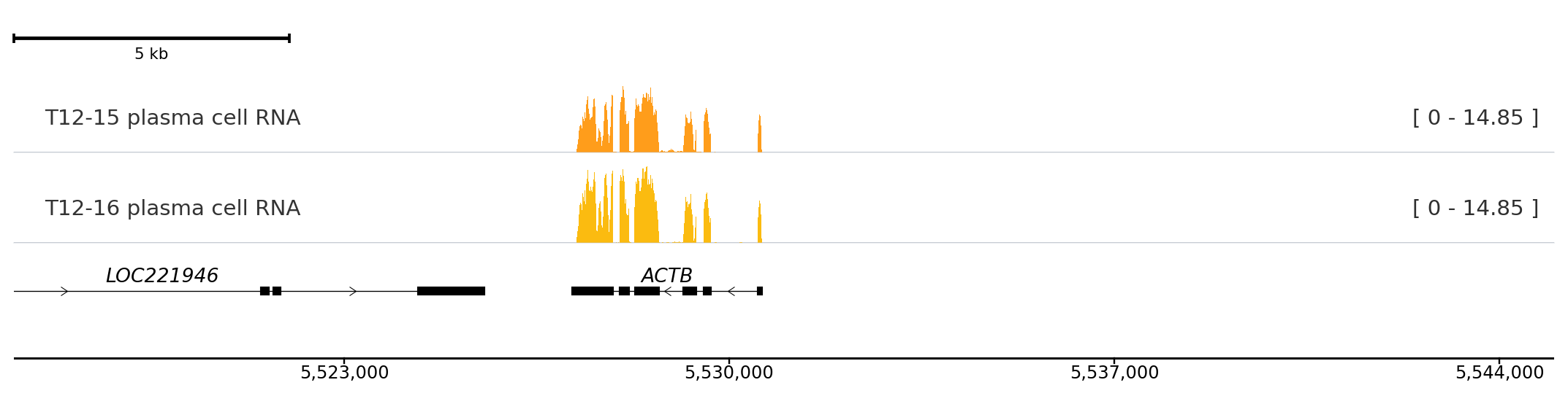
Example 1: stacked BigWig tracks with on-track labels

Two Blueprint plasma-cell RNA signal tracks rendered in separate panels with on-track label boxes and a shared autoscale group so both panels use the same y-axis limits.

fig = GenomicFigure(theme="publication")
fig.scalebar()
for name, url in BLUEPRINT_RNA_FILES.items():
    fig.bigwig(
        url,
        title=name,
        style="fragment",
        height=0.55,
        autoscale_group="blueprint_rna",
        label_on_track=True,
        label_box_enabled=True,
        label_box_alpha=0.95,
        title_height=0.5,
        scale_height=0.5,
        plot_scale=True,
    )
fig.genes("hg38", height=0.55)
fig.axis()
fig.plot(ACTB_REGION, extend=10_000)

Blueprint plasma-cell RNA at the ACTB locus. Both tracks share one autoscale group, so differences in expression level are directly comparable.

---

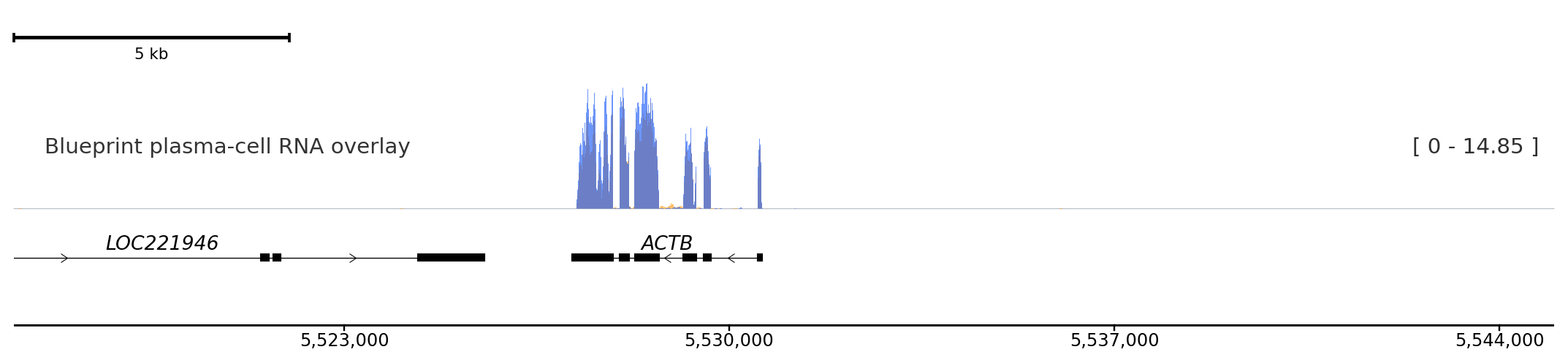
Example 2: bigwig_overlay() with a shared axis

bigwig_overlay() places multiple signals in one panel on a shared y-axis. Use this when you want to compare signal shape rather than absolute levels.

fig = GenomicFigure(theme="publication")
fig.scalebar()
fig.bigwig_overlay(
    list(BLUEPRINT_RNA_FILES.values()),
    title="Blueprint plasma-cell RNA overlay",
    colors=["#FF9D1B", "#1E5DF8"],
    alpha=0.65,
    height=0.9,
    label_on_track=True,
    label_box_enabled=True,
    label_box_alpha=0.95,
    title_height=0.5,
    scale_height=0.5,
    plot_scale=True,
    style=PlotStyle.FRAGMENT,
)
fig.genes("hg38", height=0.55)
fig.axis()
fig.plot(ACTB_REGION, extend=10_000)

Overlay of two Blueprint RNA tracks at the ACTB locus. One panel, one y-axis, colors distinguish the two samples.

---

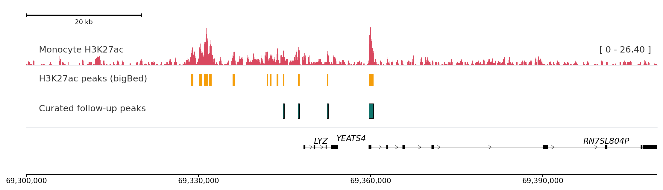
Example 3: signal + peaks + curated BED at the LYZ locus

A three-layer review plot: BigWig signal, hub peak calls from a remote BigBed, and a checked-in BED of candidate loci for follow-up.

fig = GenomicFigure(theme="publication")
fig.scalebar()
fig.bigwig(
    BLUEPRINT_MONOCYTE_BW,
    title="Monocyte H3K27ac",
    style=PlotStyle.FRAGMENT,
    height=0.6,
    color="#d9485f",
    label_on_track=True,
    label_box_enabled=True,
    label_box_alpha=0.95,
    title_height=0.5,
    scale_height=0.5,
    plot_scale=True,
)
fig.bed(
    BLUEPRINT_MONOCYTE_BB,
    title="H3K27ac peaks (bigBed)",
    color="#f59e0b",
    draw_edges=False,
    height=0.42,
    label_on_track=True,
    label_box_enabled=True,
    label_box_alpha=0.95,
    title_height=0.7,
    show_labels=False,
)
fig.bed(
    CANDIDATE_BED,
    title="Curated follow-up peaks",
    color="#0f766e",
    draw_edges=True,
    show_labels=True,
    label_field="name",
    font_size=7,
    height=0.5,
    label_on_track=True,
    label_box_enabled=True,
    label_box_alpha=0.95,
    title_height=0.7,
)
fig.genes("hg38", height=0.55)
fig.axis()
fig.plot(LYZ_REGION, extend=10_000)

Blueprint monocyte H3K27ac signal, hub peak calls, and curated candidate peaks at the LYZ locus.